Signals

a single independent variable: time Continuous-Time (CT) and Discrete-Time (DT)

Signal energy and power

signal type	energy	power
CT	\(E_{\infty}\triangleq\lim_{T\to\infty}\int_{-T}^{T}{\vert x(t)\vert}^{2}\mathrm{d}t=\int_{-\infty}^{\infty}{\vert x(t)\vert}^{2}\mathrm{d}t\)	\(P_{\infty}\triangleq\operatorname*{lim}_{T\to\infty}\frac{1}{2T}\int_{-T}^{T}{\vert x(t)\vert }^{2}\mathrm{d}t\)
DT	\(E_{\infty}\triangleq\operatorname*{lim}_{N\to\infty}\sum_{-N}^{N}{\vert x[n]\vert}^{2}=\sum_{-\infty}^{\infty}{\vert x[n]\vert}^{2}\)	\(P_{\infty}\triangleq\operatorname*{lim}_{N\to\infty}{\frac{1}{2N+1}}\sum_{-N}^{N}{\vert x[n]\vert}^{2}\)

transformation of time variable

• time shift
• time reversal
• time scaling

Example: $x(t)\to x(2-t/3)$, can be done with {shift(2), scaling(/3), reversal} or {scaling(/3), reversal, shift(6)}. Transforming time is the inverse transformation of the signal function, like pealing an onion.

Period, Even and odd signals

periodic signals: $x(t)=x(t+T)$ or $x[n]=x[n+N]$ Fundamental period: Smallest positive value of $T$ or $N$ even-odd decomposition: even part $\frac{x(t)+x(-t)}{2}$ + odd part $\frac{x(t)-x(-t)}{2}$

Complex Exponential Signals

• CT: $x(t)=Ce^{at}$
  • Real Exponential: real $C, a$. growing ($a>0$), decaying ($a<0$).
  • Periodic Complex Exponential and Sinusoidal Signals: $C=1$, imaginary $a$. $x(t)=e^{j\omega_0t}= \cos{(\omega_0t)}+j\sin{(\omega_0t)}$, whose magnitude is unity. even-odd/real-imaginary decomposition into sinusoidal signals. fundamental period $T=\frac{2\pi}{\omega_0}$.

  • General Complex Exponential Signals: $$Ce^{at}=

    C

    e^{rt}e^{j(\omega_{0}t+\theta)}=

    C

    e^{rt}\cos(\omega_{0}t+\theta)+j

    C

    e^{rt}\sin(\omega_{0}t+\theta)$$

• DT: $x[n]=C\alpha^n$
  • Real Exponential: real $C$ and $\alpha$ %这里的定义和CT不一样？振荡本来是算第三类，因为现在采样的原因?

  • Sinusoidal Signals: $

    \alpha

    =1$. $x[n]=e^{j\omega_0n}=\cos{(\omega_0n)}+j\sin{(\omega_0n)}$. fundamental period $N=\frac{2\pi m}{\omega_0}$.

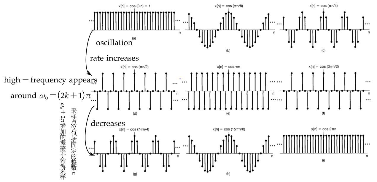
  • General Complex Exponential Signals: $$C\alpha^n\equiv

    C

    \alpha

    ^ne^{j(\omega_0n+\theta)}=

    C

    \alpha

    ^n\cos(\omega_0n+\theta)+j

    C

    \alpha

    ^n\sin{(\omega_0n+\theta)}$$

  • Special Properties due to Sampling (DT sinusoidal sequences for several different frequencies):

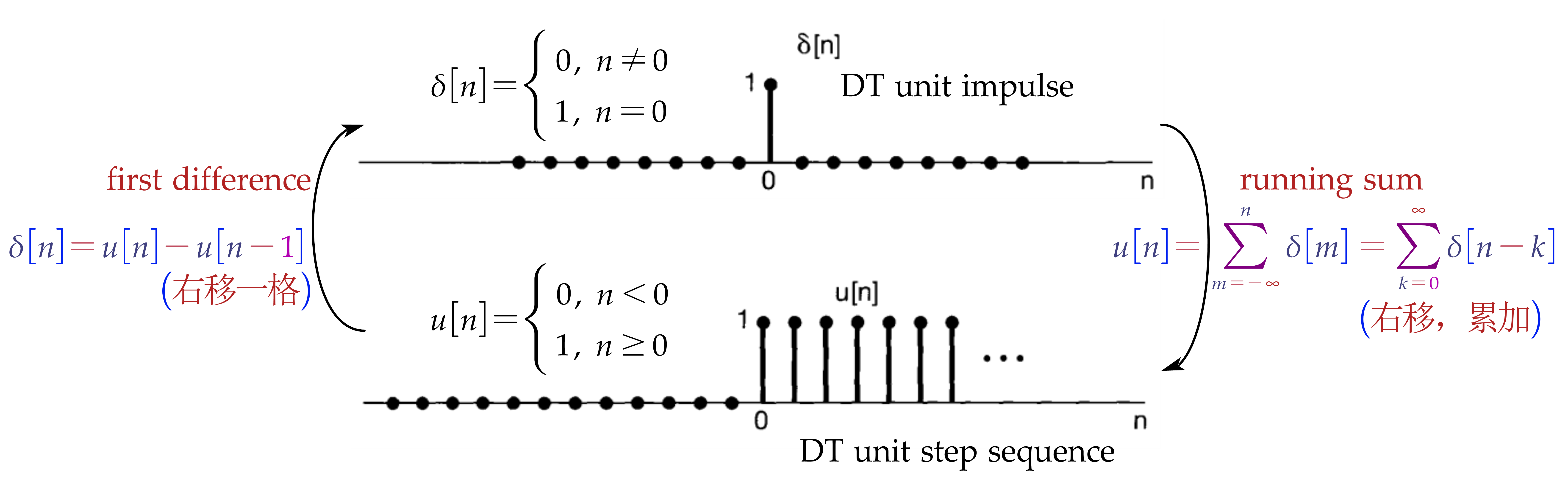
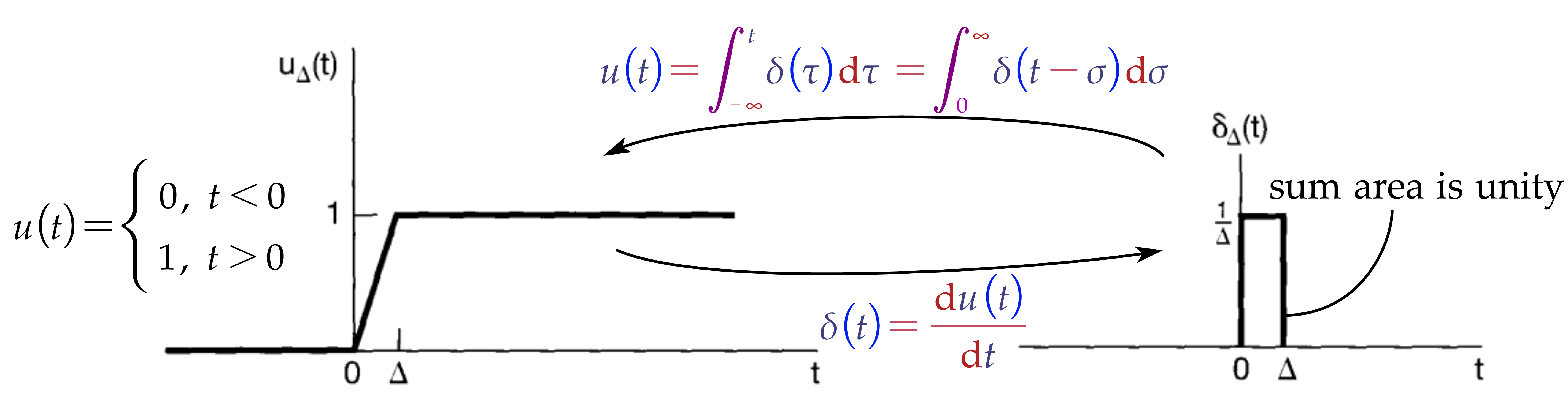
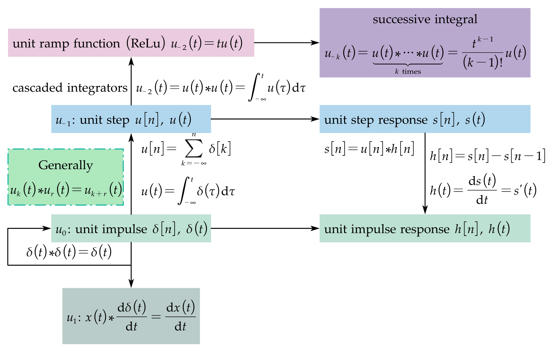
    Unit Impulse and Unit Step Functions

    

	DT	CT
sampling property 1	\(x[n]\delta[n]=x[0]\delta[n]\)	\(x(t)\delta(t)=x(0)\delta(t)\)
sampling property 2	\(x[n]\delta[n-n_0]=x[n_0]\delta[n-n_0]\)	\(x(t)\delta(t-t_0)=x(t_0)\delta(t-t_0)\)
other properties	\(x[n]=\sum^\infty_{k=-\infty}{x[k]\delta[n-k]}\)	time scaling $\delta(at)=\frac{1}{\vert a\vert}\delta(t)$

Systems

Four Basic Systems: Summer/accumulator, multiplier, differential, delay Interconnections of Systems: Series/cascade, Parallel, Series-parallel, Feedback

With and Without Memory

||memoryless|with memory| |—|—|—| |def|depend only on input at $t$|depend also on past or future value| |e.g.|$y(t)=x(t)$|$y(t)=\int_{-\infty}^t{x(\tau)\mathrm{d}{\tau}}$|

Invertibility

满秩，单射

Causality

A system is causal if the output at any time depends not on future inputs. e.g., running sum $y[n]=\sum_{-\infty}^{n}{x[k]}$ is causal, and smoothing average $y[n]=\frac{1}{2M+1}\sum_{k=-M}^M{x[n-k]}$ is anticipative (non-causal). All memoryless systems are causal.

Stability

bounded input $\rightarrow$ bounded output

Time Invariance

A system is time invariant if the behavior and characteristics of the system are fixed over time, e.g. time shifting.

Linearity

• weighted sum of input signals $\rightarrow$ superposition of their responses, $x(t)=\sum{w_ix_i(t)}\rightarrow y(t)=\sum{w_iy_i(t)}$

Linear Time-invariant System

Convolution Sum and Integral

sifting property:

• for $x[n]$
  • $\delta$ sifts through the sequence of $x[k]$ and preserves only the value when $k=n$;
  • significance: represents $x[n]$ as a superposition of shifted, scaled basic functions $\delta[n-k]$.
• for $y[n]$
  • linearity says that the response $y[n]$ to $x[n]$ is the superposition of scaled responses $h$s to $\delta$s;
  • time-invariance shows that response to $\delta[n-k]$ is the time-shifted $h[n-k]$ for all $k$, all basic responses are time-shifted versions of each other $h_k[n]=h_0[n-k]$; if not time-invariant, $h_k[n]$ can be unrelated.
  • an LTI system is completely characterised by its responses $h[n]$ to $\delta[n]$
  • visualisation: $x[k], h[n-k]$ are functions of $k$, and at each time $k$, $g[k]=x[k]h[n-k]$ represents the contribution of $x[k]$ to the output at time $n$; calculate $y[n]$ requires repeating summing $k$s for all $n$.

for LTI	DT	CT
sifting property (linear combination of shifted $\delta$)	\(x[n]=\sum_{-\infty}^{\infty}{x[k]\delta[n-k]}\)	\(x(t)=\int^\infty_{-\infty}{x(\tau)\delta(t-\tau)\mathrm{d}\tau}\)
unit impulse response (basis vector transform)	\(\delta[n]\rightarrow h[n]\)	\(\delta(t)\rightarrow h(t)\)
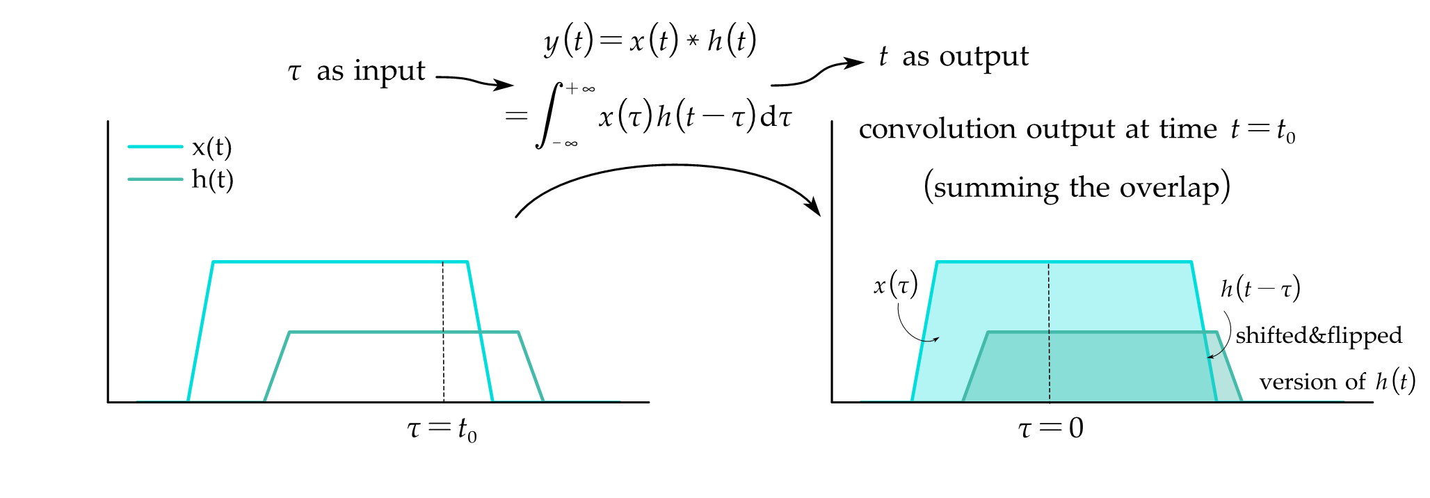
convolution output	\(\text{convolution sum}\\y[n]=x[n]*h[n]=\sum_{-\infty}^\infty{x[k]h[n-k]}\)	\(\text{convolution integral}\\y(t)=x(t)*h(t)=\int_{-\infty}^\infty{x(\tau)h(n-\tau)\mathrm{d}\tau}\)
examples		\(x(t)*u(t)=\int^t_{-\infty}{x(\tau)\mathrm{d}\tau}\\x(t)*\delta(t)=x(t)\\x(t)*\delta(t-t_0)=x(t-t_0)\)

Visualisation of Convolution:

Properties

|for LTI|DT|CT| |—|—|—| |commutative|$x[n]\ast h[n]=h[n]\ast x[n]$|$x(t)\ast h(t)=h(t)\ast x(t)$| |distributive|$x[n](h_1[n]+h_2[n])=x[n]h_1[n]+x[n]h_2[n]$|$x(t)[h_1(t)+h_2(t)]=x(t)h_1(t)+x(t)h_2(t)$| |associative|$x[n](h_1[n]h_2[n])=x[n]h_1[n]h_2[n]$|$x(t)[h_1(t)h_2(t)]=x(t)h_1(t)h_2(t)$| |without memory (nonzero only at 0)|$h[n]=K\delta[n]$|$h(t)=K\delta(t)$| |invertibility||$h(t)\ast h_1(t)=\delta(t)$| |causality|$h[n]=0, \text{for }n<0$|$h(t)=0, \text{for }t<0$| |stability|$\sum{\vert h[k]\vert}<\infty$|$\int{\vert h(\tau)\vert\mathrm{d}\tau}<\infty$|

First-order Systems described by Difference and Differential Equations

• Linear Constant-Coefficient Differential Equation: \(\sum^N_{k=0}{a_k\frac{\mathrm{d}^ky(t)}{\mathrm{d}t^k}}=\sum^M_{k=0}{b_k\frac{\mathrm{d}^kx(t)}{\mathrm{d}t^k}}\)
• Linear Constant-Coefficient Difference Equations: \(\sum^N_{k=0}{a_ky[n-k]}=\sum^M_{k=0}{b_kx[n-k]}\) specially, Recursive Equation: \(y[n]=\frac{1}{a_0}\left(\sum^M_{k=0}{b_kx[n-k]} -\sum^N_{k=1}{a_ky[n-k]}\right)\)
• Auxiliary Conditions (initial rest): the system has no output before an input
  • CT: if $x(t)=0$ for $t\le t_0$, $y(t_0)=0$
  • DT: nonrecursive equation $y[n]=\sum^M_{k=0}{\frac{b_k}{a_0}x[n-k]}$

Unit Doublets

• re-definition through convolution: unit impulse is the signal for which $x(t)=x(t)\ast \delta(t)$ for any $x(t)$.

Unit Doublets, Definition and Operations:

Fourier Series Representation of Periodic Signals

LTI System’s Response to Complex Exponentials

Complex exponentials are good signal basis for transformations. $H(s)$ is frequency response. In this case, $e^{st},z^n$ are eigenfunctions and $H(s)$ is the eigenvalue.

for CT periodic signals

basic form

• Euler’s relation: \(e^{jz}=\cos{z}+j\sin{z}, \cos{z}=\frac{e^{jz}+e^{-jz}}{2}, \sin{z}=\frac{e^{-jz}-e^{jz}}{2}\)
• set of harmonically-related complex exponetials (unit vector) \(\phi_k(t)=e^{jk\omega_0t}=e^{jk(2\pi/T)t},\quad k=0,\pm 1,\pm 2,\dots\)
• as linear combinations [Fourier Series] \(\begin{aligned} x(t)&=\sum^{+\infty}_{-\infty}{a_k\phi_k}\qquad (a_k=A_ke^{j\theta_k}=B_k+jC_k)\\&=a_0+2\sum^{+\infty}_{-\infty}{A_k\cos{(k\omega_0t+\theta_k)}}\\&=a_0+2\sum^{+\infty}_{-\infty}{(B_k\cos{(k\omega_0t)}-C_k\sin{(k\omega_0t)})} \end{aligned}\)

Synthesis and Analysis Equations

• `sifting’:\(\int_{T}e^{j(k-n)\omega_0t}\mathrm{d}t=\begin{cases} T,& k=n\\ 0,& k\neq n\\ \end{cases}\)

\[\begin{aligned} x(t)=\sum_{k=-\infty}^\infty{a_ke^{jk\omega_0t}}&\quad\begin{array}{c} [\text{synthesis}]\\ \text{freq. decompose}\\ \end{array}\\ a_k=\frac{1}{T}\int_T{x(t)e^{-jk\omega_0t}\mathrm{d}t}&\quad\begin{array}{c} [\text{analysis}]\\ \text{average/inner product}\\ \end{array} \end{aligned}\]

convergence condition

1. $x(t)$ must be absolutely integrable over any period
2. a finite number of maxima and minima in any finite time interval
3. a finite number of discontinuities and finite discontinuity in any finite time interval

Gibbs Phenomenon: Ripples at discontinuities (e.g.9\%overshoot for unit height impulse) do not decrease with an increasing $N$, which comsumpts extra energy.

Properties

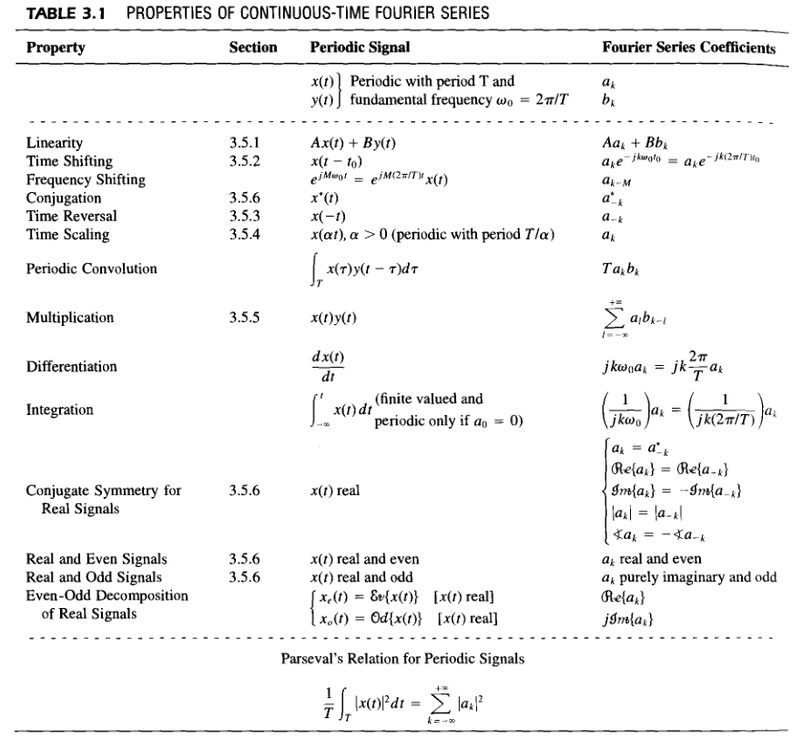Parseval’s relation: \(\text{total average power (signal)} = \sum{\text{power (harmonic component)}}\)

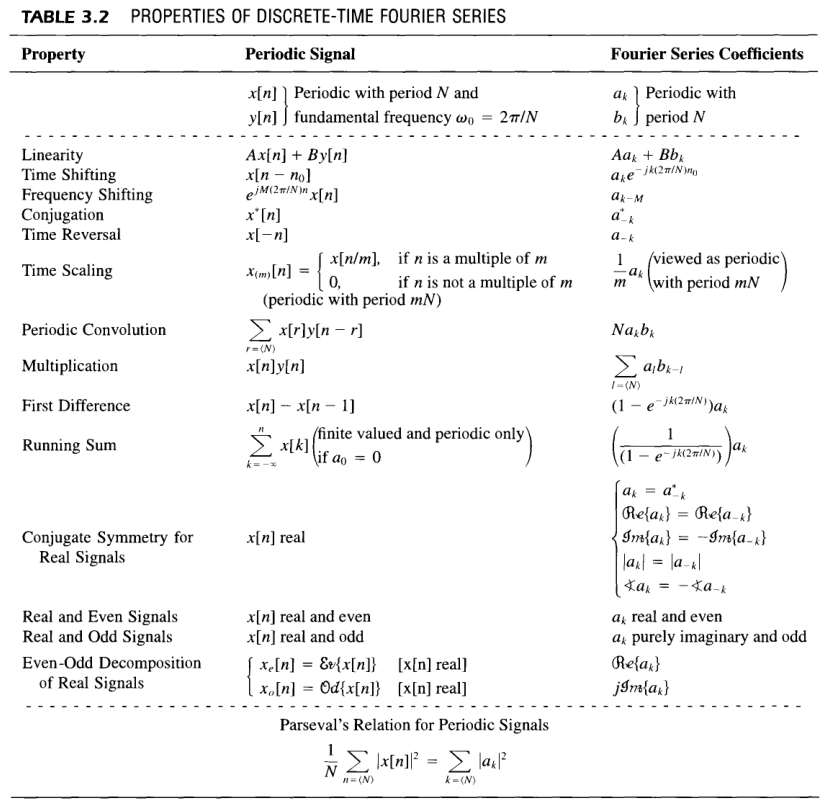
for DT signals

basic form

• sifting:\(\sum_{n=\left< N \right>}e^{jk(2\pi/N)n}=\begin{cases} N,& k=0,\pm N,\pm 2N,\dots\\ 0,& \text{otherwise}\\ \end{cases}\)
• As a consequence of the fact that DT complex exponetials whose frequencies differ by a multiple of $2\pi$ are identical ($\phi_k[n]=\phi_{k+rN}[n]$), DT Fourier series representation is a finite sequence, \(\begin{aligned} x[n]=\sum_{k=\left< N \right> }{a_ke^{jk\omega_0n}}=\sum_{k=\left< N \right> }{a_ke^{jk(2\pi/N)n}}&\quad\begin{array}{c} [\text{synthesis}]\\ \text{freq. decompose}\\ \end{array}\\ a_k=\frac{1}{N}\sum_{n=\left< N \right>}{x(t)e^{-jk\omega_0n}}=\frac{1}{N}\sum_{n=\left< N \right>}{x(t)e^{-jk(2\pi/N)n}}&\quad\begin{array}{c} [\text{analysis}]\\ \text{average/inner product} \end{array}\\ a_k=a_{k+N}&\\ \end{aligned}\)

  convergence

  In contrast to CT case, there’re no convergence issues and Gibbs phenomenon

  Properties

  

Filtering

Frequency-shaping/selective filters. use convolution to calculate output in the time domain, use filtering in the frequency domain.

Continuous-Time Fourier Transform

Fourier Transform Representation for Aperiodic Signals

Noticing that the envelope function $Ta_k$ is independent of $T$ selected but is made up of harmonic components spaced closer in frequency, we discussed that an aperiodic signal being viewed as a periodic signal whose $T\to\infty$ can be represented in a similar form to periodic signals using Fourier Transform, \(\begin{aligned} x(t)=\frac{1}{2\pi}\int_{-\infty}^{\infty}{X(j\omega)e^{j\omega t}\mathrm{d}\omega}&\quad[\text{synthesis/inverse FT}]\\ X(j\omega)=Ta_k=\int_{-\infty}^\infty{x(t)e^{-j\omega t}\mathrm{d}t}&\quad[\text{analysis/FT}] \end{aligned},\) $X(j\omega)$ is also refered to as $\mathcal{F}(x(t))$ (Fourier transform/integral/spectrum of $x(t)$). Fourier transform has the same conditions for convergence as CT fourier series representation.

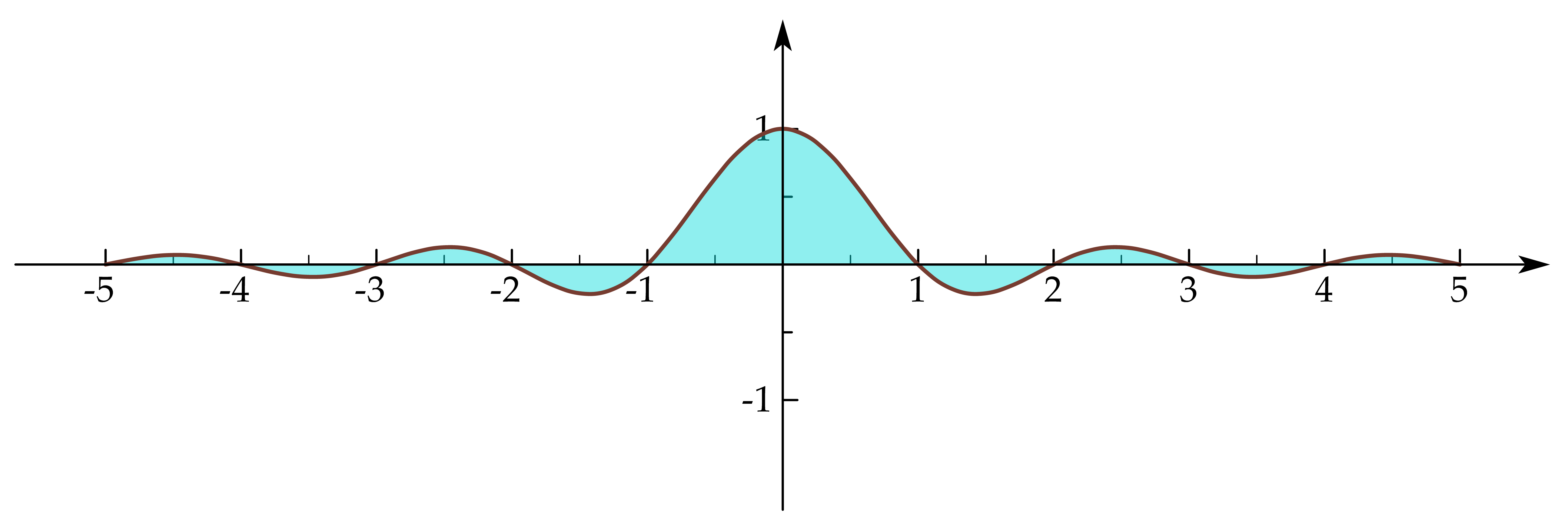
Sinc Functions

Sinc functions are related to transform of pulses (pair) \(\operatorname{sinc}(\theta)=\frac{\sin(\pi\theta)}{\pi\theta}\)

Fourier Transform for Periodic Signals

The same Fourier Transform can be applied on periodic signals, e.g. consider an impulse train which is the linear combination of shifted $2\pi\delta(\omega)$ \(X(j\omega)=\sum_{k=-\infty}^{+\infty}{2\pi a_k \delta (\omega-k\omega_0)}\leftrightarrow x(t)=\sum_{k=-\infty}^{+\infty}{a_k e^{jk\omega_0t}}\)

Properties and Basic Transform Pairs

differential equations

linear constant-coefficient differential equation and the corresponding frequency response \(\sum_{k=0}^N{a_k\frac{\mathrm{d}^ky(t)}{\mathrm{d}t^k}}=\sum_{k=0}^M{b_k\frac{\mathrm{d}^kx(t)}{\mathrm{d}t^k}}\Leftrightarrow H(j\omega)=\frac{\sum_{k=0}^M{b_k(j\omega)^k}}{\sum_{k=0}^N{a_k(j\omega)^k}}\)

Discrete-Time Fourier Transform

Fourier Transform Representation for Aperiodic Signals

The systhesis equation represents $x[n]$ as a linear combination of complex exponentials infinitesimally close in frequency and with amplitude $X(e^{j\omega}) {\frac{\mathrm{d}\omega}{2\pi}}$. The analysis equation represents $X(e^{j\omega})$ as the inner product of $x[n]$ and complex exponetials $e^{j\omega n}$ \(\begin{aligned} x[n]=\frac{1}{2\pi}\int_{2\pi}{X(e^{j\omega})e^{j\omega n} {\mathrm{d}\omega}}&\quad[\text{synthesis/inverse FT}]\\ X(e^{j\omega})=\sum_{n=-\infty}^\infty{x[n]e^{-j\omega n}}&\quad[\text{analysis/FT}] \end{aligned},\)

Fourier Transform for Periodic Signals

FT for periodic signals can be built from their Fourier coefficients. \(x[n]=\frac{1}{2\pi}\int_{-\infty}^{+\infty}{\hat{X}(e^{j\omega})e^{j\omega n} {\mathrm{d}\omega}}\) e.g. consider an impulse train which is the linear combination of shifted $2\pi\delta(\omega-\omega_0)$ \(x[n]=\sum_{k = \left<N\right>}{a_ke^{jk(2\pi/N)n}}\leftrightarrow X(e^{j\omega})=\sum_{k=-\infty}^{+\infty}{2\pi a_k \delta(\omega-\frac{2\pi k}{N})}\)

Properties and Basic Transform Pairs

periodic

The DFT is periodic with a $T=2\pi$

no Gibbs phenomenon

Time and Frequency Characterization of Signals and Systems

Magnitude-Phase Representation

• linear phase ($\angle{H}=\omega t_0, \omega n_0$): time shift; non-linear phase: distortion
• when the phase of a system is linear: signal delay = phase slope
• when the phase of a system is nonlinear: signal delay = group delay $-\frac{\mathrm{d}\angle{H}}{\mathrm{d}\omega}$ (phase slope at each freq.) $\tau(\omega)$ is the time delay for freq. $\omega$

Sampling

Sampling Theorem (ideal sampling)

The samples $x(nT)$ are frequency-shifted versions of $x(t)$. For a band-limited signal $x(t)$, If $\omega_s>2\omega_M$, where $\omega_s=\frac{2\pi}{T}$, then $x(t)$ is uniquely defined by $x(nT)$ (the signal can be reconstructed). $2\omega_M$ is the Nyquist rate. There’re special cases where a sampling rate smaller than $2\omega_M$ can sample without loss.

Aliasing

When the sampling frequency $\omega_s$ is less than the Nyquist rate, the individual terms of the duplicated $X(j\omega)$ will overlap. The signal will no longer be reconstructed by lowpass filters.

Communication Systems

transmitter modulate -> receiver demodulate -> filter

Amplitude Modulation

1. double-sideband: inefficient use of BW
2. single-sideband: use filter/$90^\circ$ phase-shift network to retain USB/LSB

Demodulation

1. synchronous: transmitter and receiver synchronous in phase
2. asynchronous

Multiplexing

1. frequency-division
2. time-division

ROC

ROC is the region where $x(t)$ is integrable over time duration

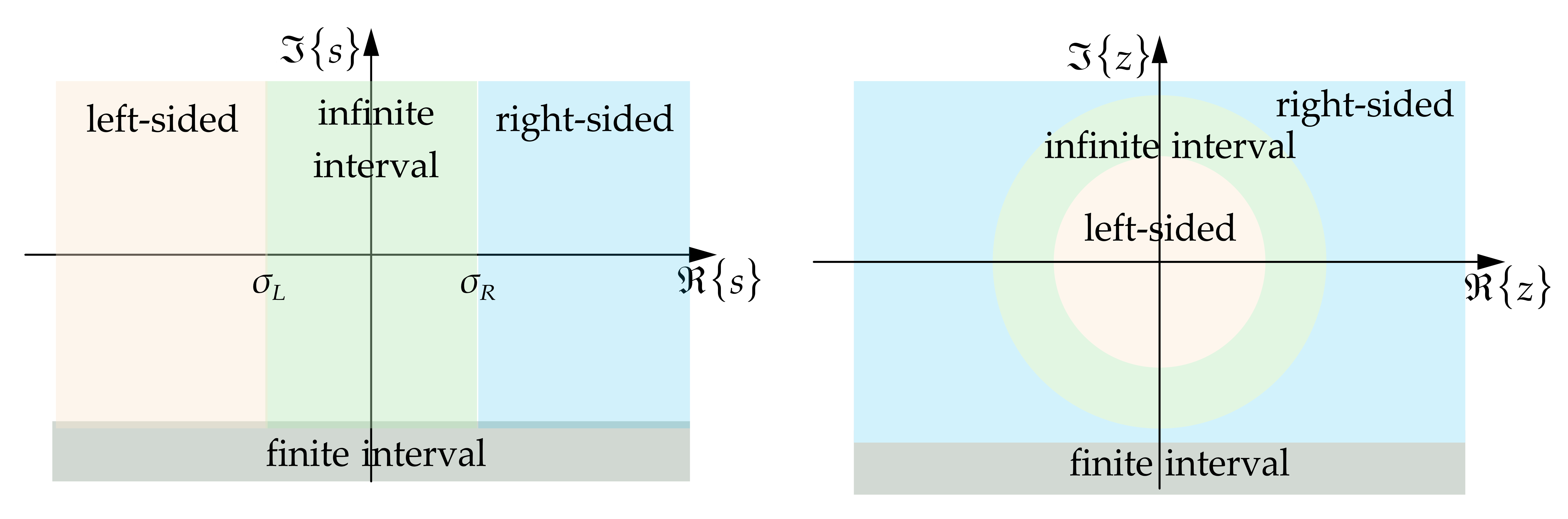
1. ROC contains no poles for rational Laplace transform. There can be several possible ROC bounded by the same set of poles.
2. FT of $x(t)$ converges when its ROC includes the $j\omega$-axis ($\sigma=0$)

   LCCDEs, unilateral transforms are causal, right-sided

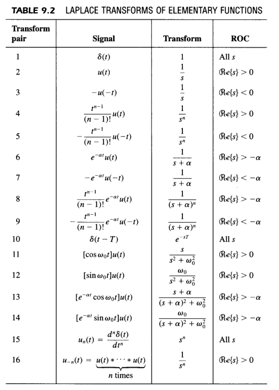
Laplace Transform

\[H(s)=\int^\infty_{-\infty}{h(t)e^{-st}\mathrm{d}t}=\int^\infty_{-\infty}{[h(t)e^{-\sigma t}]e^{-j\omega t}\mathrm{d}t}, \Re{\left\{s\right\}}\in \text{ROC} \\ x(t)=\frac{1}{2\pi j}\int^{\sigma+j\infty}_{\sigma-j\infty}{X(s)e^{st}\mathrm{d}s}\]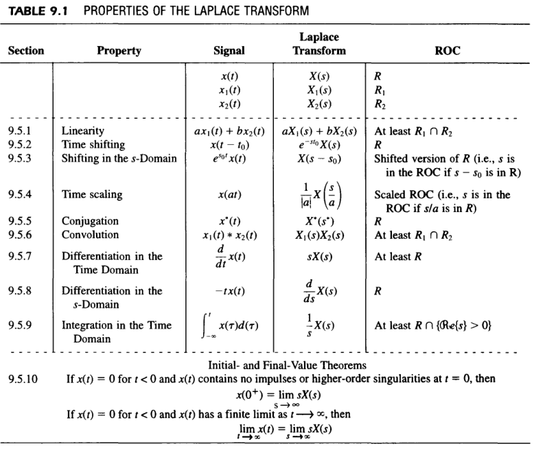

LTI Systems Using the Laplace Transform

1. causality: $h(t)=0, t<0\rightarrow \text{right-sided}$

   If the ROC of $H(s)$ is a right-half plane, the system is causal only when $H(s)$ is rational

2. stability: $H(s)$ contains $j\omega$-axis, FT exists

   a causal system with rational $H(s)$ is stable $\rightleftarrows$ no RHP poles

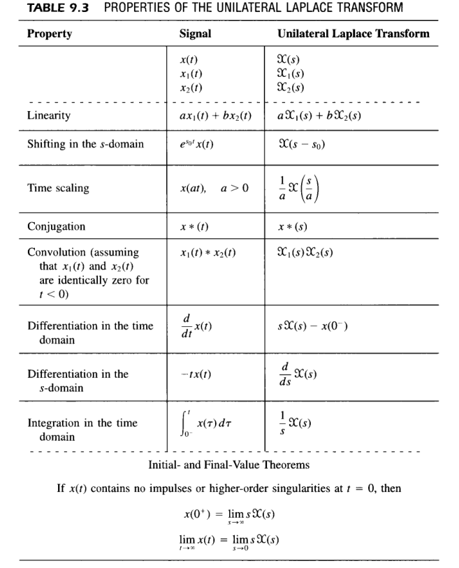
Unilateral Laplace Transform

\(\mathcal{X}(s)=\int_{0^-}^\infty x(t)e^{-st}\mathrm{~d}t=\mathcal{UL}\{x(t)\}=\mathcal{L}\{x(t)u(t^-)\}\) all properties are the same except for differentiation and convolution

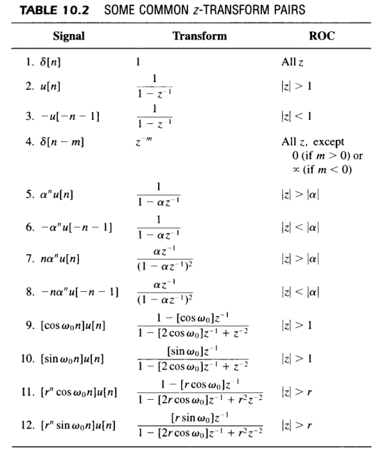
Z-Transform

\(X(z)=\sum^\infty_{n=-\infty}{x[n]z^{-n}}\)

$X(z)=X(re^{j\omega})=\mathcal{x[n]r^{-n}}$

LTI Systems Using Z-Transform

1. causality: $h(t)=0, t<0\rightarrow \text{exterior, including}\infty$;

   A DT LTI system with rational $H(z)$ is causal if and only if (a) ROC is the exterior region or (b) the polynomial ratio converges at $

   z

   =\infty$

2. stability: $H(z)$ contains unit circle $	z	=1$
   > a causal system with rational $H(z)$ is stable $\rightleftarrows$ no $	z	>1$ poles

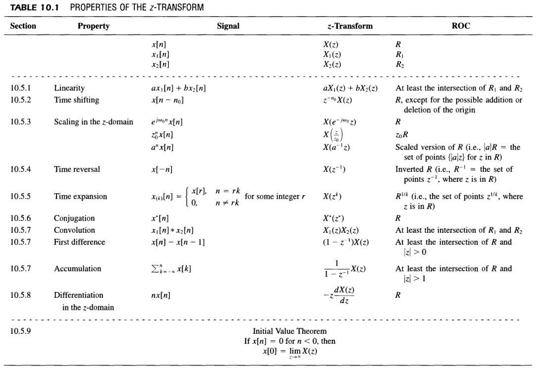
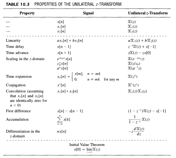
Unilateral Z-Transform

\(\mathcal{X}(z)=\sum^\infty_{n=0}{x[n]z^{-n}}=\mathcal{Z}\{x[n]u[n]\}\) time-shifting is different

Linear Constant-Coefficient Differential Equations

• \[\sum_{k=0}^Na_k\frac{\mathrm{d}^ky(t)}{\mathrm{d}t^k}=\sum_{k=0}^Mb_k\frac{\mathrm{d}^kx(t)}{\mathrm{d}t^k}\rightarrow\sum_{k=0}^Na_ks^kY(s)=\sum_{k=0}^Mb_ks^kX(s)\\ \rightarrow H(s)=\frac{Y(s)}{X(s)}=\frac{\sum_{k=0}^Mb_ks^k}{\sum_{k=0}^Na_ks^k}\]

  to solve CT causal systems (LCCDE with initial conditions $x(t)\neq 0, t<0$). take unilateral of LCCDE on both sides $\mathcal{UL}{\text{solution}}=\text{zero-input response} f(y(0^-),y^\prime(0^-),\dots)+\text{zero-state response} \mathcal{L}{x(t)}$

• \[\sum^N_{k=0}{a_ky[n-k]}=\sum^M_{k=0}{b_kx[n-k]}\rightarrow H(z)=\frac{\sum^M_{k=0}b_kz^{-k}}{\sum^N_{k=0}{a_kz^{-k}}}\]

  to solve DT causal systems (LCCDE with initial conditions). take unilateral of LCCDE on both sides

Block diagram Form

• feedback interconnection: $H(s)=\frac{A}{1-\beta A}$
• direct form: $H(s)=\frac{1}{(s+5)s+6}$ 左右/上下分离即分子与分母
• parallel form: $H(s)=\frac{1}{s+2}-\frac{1}{s+3}$
• cascade form: $H(s)=\frac{1}{s+2}\frac{1}{s+3}$